Lecture 11: Attention Layer
36th International Summer School SAA
University of Lausanne
Attention layers are fundamental components of the Transformer architecture, which has achieved remarkable success across a wide range of tasks. This notebook introduces the core concepts of attention and further explores multi-head attention along with other essential building blocks of the Transformer architecture, including time-distributed feed-forward neural networks, dropout layers, and normalization layers.
1 Attention layer
Attention layers were introduced in the seminal paper of Vaswani et al. (2017).
Attention layers were first designed for sequential data (e.g., time-series).
The starting point is an input sequence of elements:
\[ \boldsymbol{X}_{1:t} = \big[ \boldsymbol{X}_1, \, \, \dots, \, \boldsymbol{X}_t \big]^\top \in \mathbb{R}^{t \times q}, \]
where:
- \(t\) is length of the sequence,
- \(q\) is dimension of the series,
- \(\boldsymbol{X}_u \in \mathbb{R}^q\) is the \(u\)-th element of the sequence, with \(1 \leq u \leq t\).
2 Query, Key and Value
In order to be applied, an attention layer requires the following elements:
- Queries \(\boldsymbol{q}_u \in \mathbb{R}^q,\; 1 \leq u \leq t\)
- The query \(\boldsymbol{q}_u\) represents what the \(u\)-th element is trying to find in the overall input
- Act like a question asking: “What information is relevant to me?”
- The query \(\boldsymbol{q}_u\) represents what the \(u\)-th element is trying to find in the overall input
- Keys \(\boldsymbol{k}_u \in \mathbb{R}^q,\; 1 \leq u \leq t\).
- The key \(\boldsymbol{k}_u\) describes what the \(u\)-th element can provide to others.
- Function like a label indicating: “This is the kind of information I carry”.
- The key \(\boldsymbol{k}_u\) describes what the \(u\)-th element can provide to others.
- Values \(\boldsymbol{v}_u \in \mathbb{R}^q,\; 1 \leq u \leq t\)
- The value \(\boldsymbol{v}_u\) contains the actual content that can be shared
- When a query matches a key, the corresponding value is passed along as useful context.
- The value \(\boldsymbol{v}_u\) contains the actual content that can be shared
The query \(\boldsymbol{q}_u\) tries to find a key \(\boldsymbol{k}_s\) that gives a match. E.g., in a sentence the query of the subject ‘car’ tries to find a verb ‘accelerate’ in the sentence, which then gives a match for a dangerous driving maneuver. In that case, a high attention is paid to the corresponding value \(\boldsymbol{v}_s\).
Queries, keys and values are represented by the three matrices \[\begin{eqnarray*} Q &=& \left[\boldsymbol{q}_1, \ldots, \boldsymbol{q}_t\right]^\top \in \mathbb{R}^{t \times q}, \\ K &=& \left[\boldsymbol{k}_1, \ldots, \boldsymbol{k}_t\right]^\top \in \mathbb{R}^{t \times q}, \\ V &=& \left[\boldsymbol{v}_1, \ldots, \boldsymbol{v}_t\right]^\top \in \mathbb{R}^{t \times q}. \end{eqnarray*}\]
In self-attention models, \(Q\), \(K\), and \(V\) are derived from the input sequence \(\boldsymbol{X}_{1:t}\) by applying some time -distributed layers.
2.1 Time-distributed layer
Consider a time-distributed FNN layer with \(q_1\) units applied to the input tensor \(\boldsymbol{X}_{1:t} \in \mathbb{R}^{t \times q}\).
This performs the mapping \[\begin{eqnarray*} \boldsymbol{z}^{\mathrm{t\text{-}FNN}}&:& \mathbb{R}^{t \times q} \to \mathbb{R}^{t \times q_1}, \\&& \boldsymbol{X}_{1:t} \mapsto \boldsymbol{z}^{\mathrm{t\text{-}FNN}} (\boldsymbol{X}_{1:t}) = \left( \boldsymbol{z}^{\mathrm{FNN}}(\boldsymbol{X}_1), \ldots, \boldsymbol{z}^{\mathrm{FNN}}(\boldsymbol{X}_t) \right)^\top, \end{eqnarray*}\] where \(\boldsymbol{z}^{\mathrm{FNN}}: \mathbb{R}^q \to \mathbb{R}^{q_1}\) is a FNN layer.
This transformation leaves the time dimension \(t\) unchanged.
Important, the same parameters (network weights and biases) are shared across all time steps \(1\le u \le t\). This makes the FNN layer a so-called time-distributed one.
To derive \(\boldsymbol{q}_u\), \(\boldsymbol{k}_u\), and \(\boldsymbol{v}_u\), three time-distributed \(q\)-dimensional FNNs \[ \boldsymbol{z}_\kappa^{\text{t-FNN}} : \mathbb{R}^{t \times q} \to \mathbb{R}^{t \times q}, \qquad \boldsymbol{X}_{1:t} \mapsto \boldsymbol{z}_\kappa^{\text{t-FNN}}(\boldsymbol{X}_{1:t}), \] for \(\kappa =Q, K, V\), where applied.
These give us the time-slices for fixed time points \(1 \le u \le t\) \[ \begin{aligned} \boldsymbol{q}_u &= \boldsymbol{z}^{\text{FNN}}_Q(\boldsymbol{X}_u) = \phi_Q \left( \boldsymbol{w}_0^{(Q)} + W^{(Q)} \boldsymbol{X}_u \right) \in \mathbb{R}^q, \\ \boldsymbol{k}_u &= \boldsymbol{z}^{\text{FNN}}_K(\boldsymbol{X}_u) = \phi_K \left( \boldsymbol{w}_0^{(K)} + W^{(K)} \boldsymbol{X}_u \right) \in \mathbb{R}^q, \\ \boldsymbol{v}_u &= \boldsymbol{z}^{\text{FNN}}_V(\boldsymbol{X}_u) = \phi_V \left( \boldsymbol{w}_0^{(V)} + W^{(V)} \boldsymbol{X}_u \right) \in \mathbb{R}^q, \end{aligned}\] with corresponding network weights, biases, and activation functions.
Equivalently, this reads in matrix notation as \[ \begin{aligned} Q &= \boldsymbol{z}^{\text{t-FNN}}_Q(\boldsymbol{X}_{1:t}) = \left[ \boldsymbol{q}_1, \ldots, \boldsymbol{q}_t \right]^\top \in \mathbb{R}^{t \times q}, \\ K &= \boldsymbol{z}^{\text{t-FNN}}_K(\boldsymbol{X}_{1:t}) = \left[ \boldsymbol{k}_1, \ldots, \boldsymbol{k}_t \right]^\top \in \mathbb{R}^{t \times q}, \\ V &= \boldsymbol{z}^{\text{t-FNN}}_V(\boldsymbol{X}_{1:t}) = \left[ \boldsymbol{v}_1, \ldots, \boldsymbol{v}_t \right]^\top \in \mathbb{R}^{t \times q}. \end{aligned}\]
3 Attention head
The attention head is defined by the mapping \[ H: \mathbb{R}^{t \times q} \times \mathbb{R}^{t \times q} \times \mathbb{R}^{t \times q} \to \mathbb{R}^{t \times q}, \qquad (Q,K,V) \mapsto H = H(Q, K, V), \] with scaled dot-product attention \[ H = A\,V = \operatorname{softmax}\left(\frac{Q K^{\top}}{\sqrt{q}}\right) V \in \mathbb{R}^{t \times q}.\]
The attention matrix \(A \in \mathbb{R}^{t \times t}\) is obtained by applying the softmax function row-wise to matrix \(A' = QK^\top / \sqrt{q}\), that is, \[ A = \operatorname{softmax}(A'), \qquad \text{where} \quad a_{u,s} = \frac{\exp(a'_{u,s})}{\sum_{k=1}^{t} \exp(a'_{u,k})} \in (0,1). \]
This ensures that the rows sums of \(A\) are equal to one.
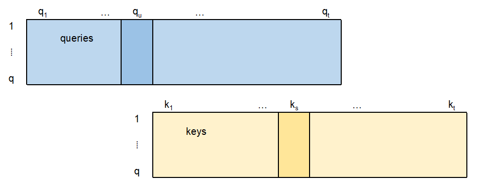
Recalling the notation \[ Q = \left[\boldsymbol{q}_1, \ldots, \boldsymbol{q}_t\right]^\top \in \mathbb{R}^{t \times q} \quad \text{and} \quad K = \left[\boldsymbol{k}_1, \ldots, \boldsymbol{k}_t\right]^\top \in \mathbb{R}^{t \times q}, \] the elements \(a'_{u,s}\) of matrix \(A'\) are given by the dot-product \[ a'_{u,s} = \frac{1}{\sqrt{q}}\, \boldsymbol{q}_u^\top \boldsymbol{k}_s = \frac{1}{\sqrt{q}}\, \left\langle \boldsymbol{q}_u, \boldsymbol{k}_s \right\rangle= \boldsymbol{q}_u \cdot \boldsymbol{k}_s/\sqrt{q}.\] These are three different ways to express the scalar product between the query \(\boldsymbol{q}_u\) and the key \(\boldsymbol{k}_s\); see also next graph.
The scaling factor \(\sqrt{q}\) removes the input dimension dependence. I.e., it prevents the dot-product operation from being too flat or too spiky.
Each entry of the attention head \(H=A\,V\) is a weighted average of the columns of the value matrix \(V\). The weights \(a_{u,s}\) determine the importance of each row vector \(\boldsymbol{v}_s\) of \(V\); see next illustration.
If the query \(\boldsymbol{q}_u\) points into the same direction as the key \(\boldsymbol{k}_s\), we receive a large attention weight \(a_{u,s}\). This implies that the corresponding entry \(\boldsymbol{v}_s\) on the \(s\)-th row of the value matrix \(V\) receives a big attention.
I.e., the information \(\boldsymbol{v}_s\) at time \(s\) is important for period \(u\) (the query \(\boldsymbol{q}_u\) at time \(u\)).
4 Multi-head Attention
The multi-head attention mechanism applies \(n_h \ge 2\) parallel attention heads to \(\boldsymbol{X}_{1:t}\).
Assume the \(j\)-th attention head is given by the query, key and value \(Q_j\), \(K_j\), and \(V_j\), respectively, defining the \(j\)-th attention head \[ H_j=H_j(\boldsymbol{X}_{1:t}) = \operatorname{softmax}\left(\frac{Q_j K_j^\top}{\sqrt{q}}\right) V_j \in \mathbb{R}^{t \times q}. \]
These heads are concatenated and linearly transformed \[ H_{\text{MH}}(\boldsymbol{X}_{1:t}) = \operatorname{Concat}\left(H_1, H_2, \dots, H_{n_h}\right) W \in \mathbb{R}^{t \times q}, \] for an output weight matrix \(W \in \mathbb{R}^{n_hq \times q}\).
This multi-head attention is further processed as described above.
5 Other Layers in Transformers
In addition to attention and feed-forward components, transformer architectures also commonly include:
- Layer Normalization
- Helps stabilize and speed up training by reducing internal covariate shift.
- Drop-out Layer
- Used as a regularization technique to prevent overfitting.
5.1 Layer normalization
Layer normalization is a mapping \[ \boldsymbol{z}^{\text{norm}} : \mathbb{R}^{q} \to \mathbb{R}^{q}, \qquad \boldsymbol{X} \mapsto \boldsymbol{z}^{\text{norm}} ( \boldsymbol{X}) = \left( \gamma_j \left( \frac{ {X}_j - \bar{X}}{\sqrt{s^2 + \epsilon}} \right) + \delta_j\right)_{1\le j \le q},\] where \(\epsilon > 0\) is a small constant added for numerical stability.
The empirical mean \(\bar{X} \in \mathbb{R}\) and variance \(s^2 \in \mathbb{R}^+\) are computed as \[ \bar{X}= \frac{1}{{q}} \sum_{j=1}^{q} X_j \qquad \text{ and } \qquad s^2 = \frac{1}{q} \sum_{j=1}^{q} (X_j - \bar{X})^2.\]
\(\boldsymbol{\gamma} = (\gamma_1, \ldots, \gamma_{q})^\top \in \mathbb{R}^{q}\) and \(\boldsymbol{\delta} = (\delta_1, \ldots, \delta_{q})^\top \in \mathbb{R}^{q}\) are vectors of trainable parameters.
5.2 Drop-out layer
Drop-out has been introduced by Srivastava et al. (2014) and Wager, Wang and Liang (2013).
Drop-out is typically implemented by multiplying the output of a specific layer by i.i.d. realizations of Bernoulli random variables with a fixed drop-out rate \(\alpha \in (0,1)\) in each step of SGD training.
Drop-out is formalized by \[ \boldsymbol{z}^{\text{drop}} : \mathbb{R}^{q} \to \mathbb{R}^{q}, \qquad \boldsymbol{X} \mapsto \boldsymbol{z}^{\text{drop}}( \boldsymbol{X}) = \boldsymbol{Z} \odot \boldsymbol{X},\] where \(\boldsymbol{Z} = (Z_1, Z_2, \ldots, Z_{q})^\top \in \{0, 1\}^{q}\) is a vector of i.i.d. Bernoulli random variables that are re-sampled in each SGD step, and \(\odot\) denotes the element-wise Hadamard product.